BRIEF: Lagrange Multipliers

Find the maximum value of

\[f(x,y,z) = x^2 + y^2 - z\]

subject to the constraint

\[x + y - 2z = 0\]

The function f maps a subset of $\mathbb{R}^3$ to real values in $\mathbb{R}$, and the constraint is a level set of a similar function $g$. What is a level set, you might ask? Great question. A level set of a function is a collection of all input points that give the same output.

Example: Consider the function $f(x,y) = x2 + y2$. Which set of inputs $(x,y)$ make $f(x,y) = 4$?

You have seen $x^2 + y^2 = 4$, and other equations like it. As shown in the graph below, where $f(x,y)$ is blue, when we set our function equal to a given value, we get the set of points that output that value. The actual level set exists on the x-y plane, but for the sake of visualization, I have included both the level set and the level set projected onto $f$’s surface.

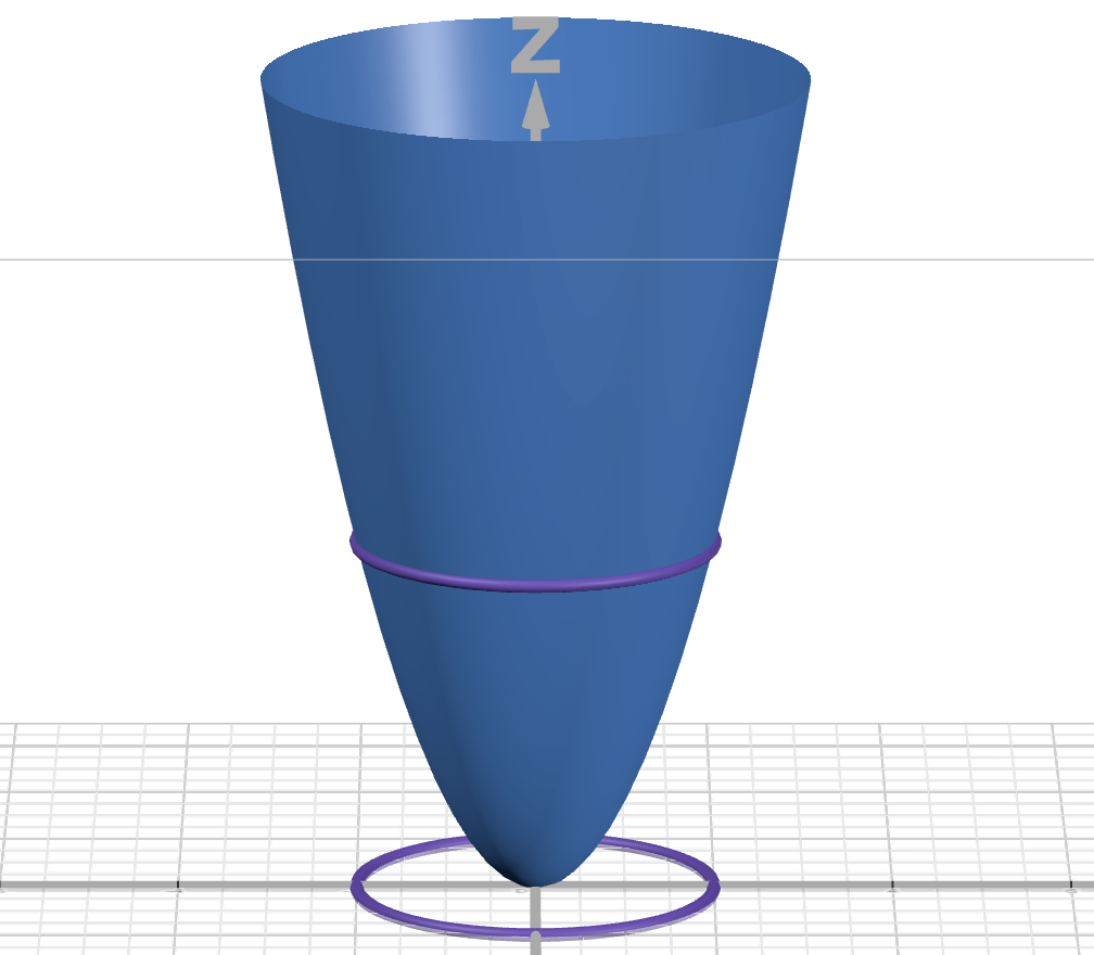
In this case, our function’s graph is a surface, and the level set is a curve.

Note: The surface is a 2D object in 3D, and the curve is a 1D object in 2D.

Going back to our original problem, $g$ is the function $g(x,y,z) = x + y - 2z$. Our specific constraint is the level set of this function where $g(x,y,z) = 0$. Rather than a curve, this gives us a surface.

We want to find the maximum output of $f(x,y,z)$ subject to this constraint. All points $(x,y,z)$ that reach that maximum output form a level surface of $f$, though we only care about points that also satisfy the constraint.

We solve our problem by finding the level sets of $f$ associated with the maximum value.

There are many possible level sets of $f$. For this problem, changing what the level set is equal to moves the surface up and down, but for other formulas, it can change the surface in different ways.

If we have a point of intersection between our level set and constraint surface that is not a tangent point between the two surfaces, we can move our level set while still having overlap, meaning there are solutions with higher and lower $f$ values. Therefore, this is not an optimized point. Only tangent and boundary points can be maximums or minimums.

We have successfully restructured the goal of our problem: we want to find level sets of $f$ that are tangent to our constraint surface.

How do we do that? We find points where the two gradients are parallel. If you don’t know what a gradient is, think of it as a higher-dimensional derivative. The gradient of a function is perpendicular to its level surface.

Therefore, if a level surface is tangent to the constraint surface, their gradients will be parallel:

\[\nabla f = \lambda \nabla g\]

When the gradients are parallel, we can multiply $\nabla g$ by an unknown scalar ($\lambda$, the Lagrange multiplier), making it equal to $\nabla f$.

To ensure our points lie on our constraint surface, we add the original constraint equation to our system. Every point p already lies on the level surface $f = f(p)$.

The points that satisfy this system of equations are on both surfaces, and we know those surfaces are parallel. Therefore, the surfaces must be tangent at these points.

To solve this problem, we calculate the gradients and set them equal to each other, multiplying $\nabla g$ by a Lagrange multiplier. Together with the constraint equation, this forms a system of equations. The solutions to this system of equations are potential candidates for the maximum or minimum points. We can use these to find true extrema.

That’s pretty boring, so I wrote some code to do it. (GitHub)

The maximum of our original problem is -1/8, occurring at (1/4, 1/4, 1/4).

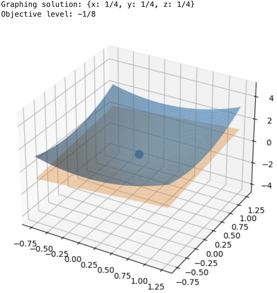
Let’s look at a different problem:

Find the maximum and minimum values of $f(x,y,z)=xyz$ subject to the constraint $x + 9y^2 + z^2 = 36$. Assume that $x ≥ 0$. (We must assume so, or there will be no absolute extrema)

For this problem:

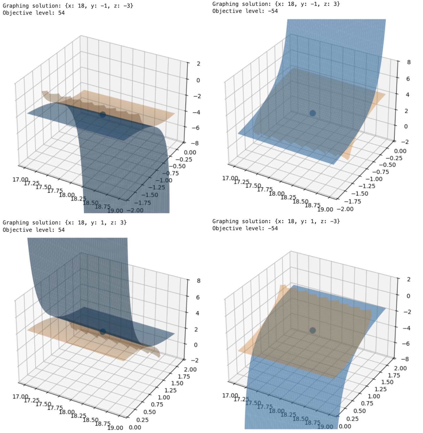
We reach a maximum of 54 at points (18, -1, -3) and (18, 1, 3).

We reach a minimum of -54 at points (18, -1, 3) and (18, 1, -3).

Having multiple max or min points means that at the optimal level set, there happen to be multiple tangent points. Solution points shown below:

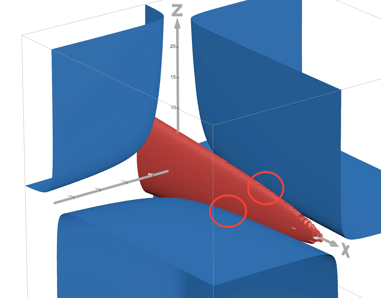
The two maximum tangent points in Desmos, for context. Cool.

These problems come up fairly often. For example, they are used in the constrained optimization problem behind support vector machines, a fundamental machine learning model: Caltech lecture.

You can use Lagrange multipliers to solve optimization problems in 2D, 4D, or any number of dimensions. You can also solve problems with multiple constraints. The visualization only works for 3d, but if you want, you can use the calculator to mess around with higher-dimensional optimization problems. (Again: GitHub link)