subject to the constraint

The function f maps a subset of $\mathbb{R}^3$ to real values in $\mathbb{R}$, and the constraint is a level set of a similar function $g$. What is a level set, you might ask? Great question. A level set of a function is a collection of all input points that give the same output.

Example: Consider the function $f(x,y) = x2 + y2$. Which set of inputs $(x,y)$ make $f(x,y) = 4$?

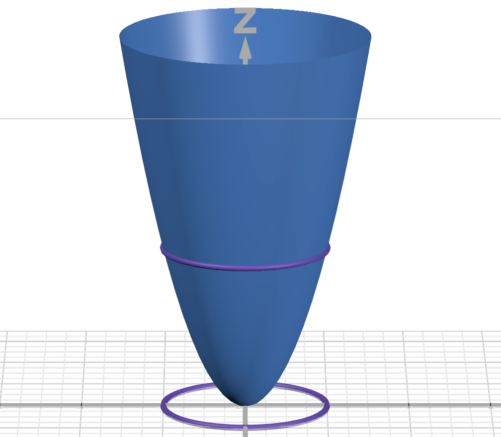
You have seen $x^2 + y^2 = 4$, and other equations like it. As shown in the graph below, where $f(x,y)$ is blue, when we set our function equal to a given value, we get the set of points that output that value. The actual level set exists on the x-y plane, but for the sake of visualization, I have included both the level set and the level set projected onto $f$’s surface.

In this case, our function’s graph is a surface, and the level set is a curve.

Note: The surface is a 2D object in 3D, and the curve is a 1D object in 2D.

Going back to our original problem, $g$ is the function $g(x,y,z) = x + y - 2z$. Our specific constraint is the level set of this function where $g(x,y,z) = 0$. Rather than a curve, this gives us a surface.

We want to find the maximum output of $f(x,y,z)$ subject to this constraint. All points $(x,y,z)$ that reach that maximum output form a level surface of $f$, though we only care about points that also satisfy the constraint.

We solve our problem by finding the level sets of $f$ associated with the maximum value.

There are many possible level sets of $f$. For this problem, changing what the level set is equal to moves the surface up and down, but for other formulas, it can change the surface in different ways.

If we have a point of intersection between our level set and constraint surface that is not a tangent point between the two surfaces, we can move our level set while still having overlap, meaning there are solutions with higher and lower $f$ values. Therefore, this is not an optimized point. Only tangent and boundary points can be maximums or minimums.

We have successfully restructured the goal of our problem: we want to find level sets of $f$ that are tangent to our constraint surface.

How do we do that? We find points where the two gradients are parallel. If you don’t know what a gradient is, think of it as a higher-dimensional derivative. The gradient of a function is perpendicular to its level surface.

Therefore, if a level surface is tangent to the constraint surface, their gradients will be parallel:

When the gradients are parallel, we can multiply $\nabla g$ by an unknown scalar ($\lambda$, the Lagrange multiplier), making it equal to $\nabla f$.

To ensure our points lie on our constraint surface, we add the original constraint equation to our system. Every point p already lies on the level surface $f = f(p)$.

The points that satisfy this system of equations are on both surfaces, and we know those surfaces are parallel. Therefore, the surfaces must be tangent at these points.

To solve this problem, we calculate the gradients and set them equal to each other, multiplying $\nabla g$ by a Lagrange multiplier. Together with the constraint equation, this forms a system of equations. The solutions to this system of equations are potential candidates for the maximum or minimum points. We can use these to find true extrema.

That’s pretty boring, so I wrote some code to do it. (GitHub)

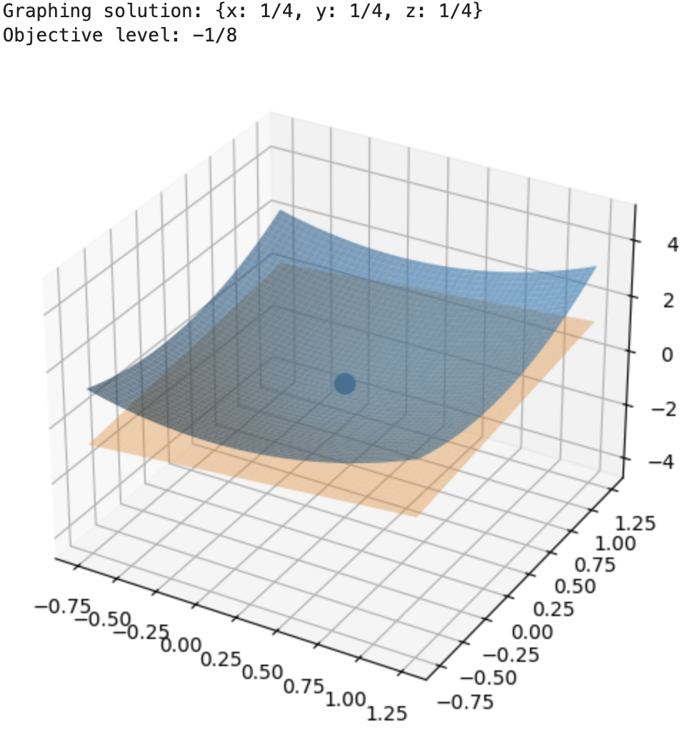
The maximum of our original problem is -1/8, occurring at (1/4, 1/4, 1/4).

Let’s look at a different problem:

Find the maximum and minimum values of $f(x,y,z)=xyz$ subject to the constraint $x + 9y^2 + z^2 = 36$. Assume that $x ≥ 0$. (We must assume so, or there will be no absolute extrema)

For this problem:

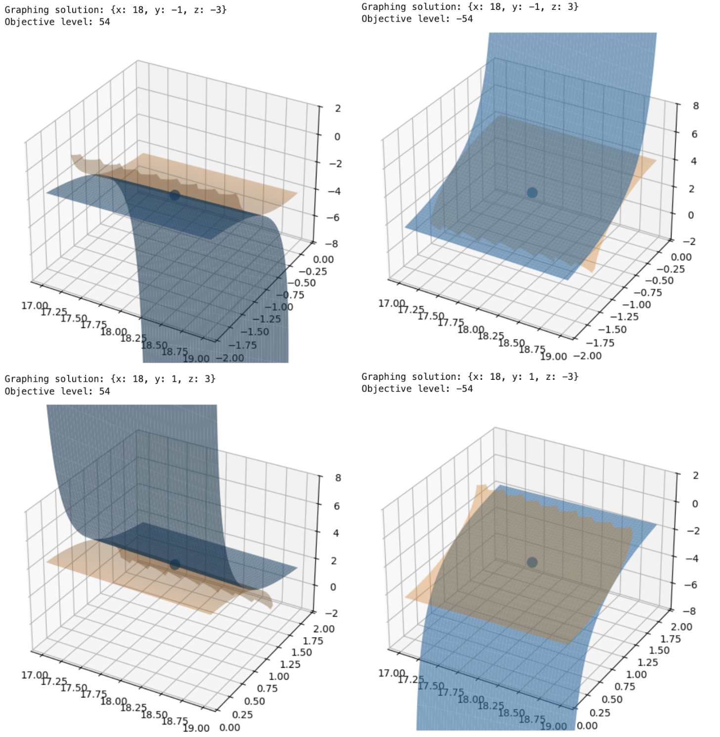
We reach a maximum of 54 at points (18, -1, -3) and (18, 1, 3).

We reach a minimum of -54 at points (18, -1, 3) and (18, 1, -3).

Having multiple max or min points means that at the optimal level set, there happen to be multiple tangent points. Solution points shown below:

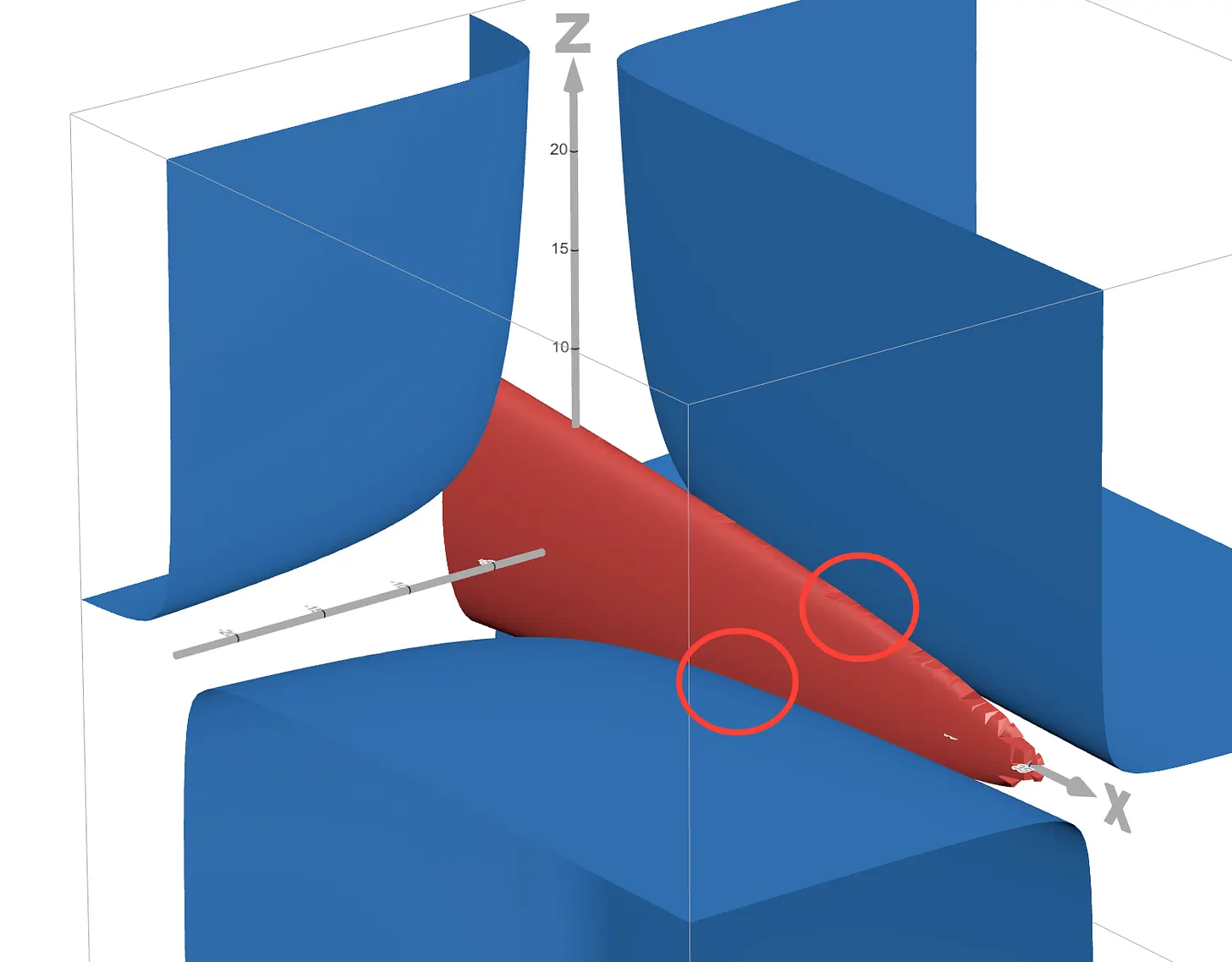
The two maximum tangent points in Desmos, for context. Cool.

These problems come up fairly often. For example, they are used in the constrained optimization problem behind support vector machines, a fundamental machine learning model: Caltech lecture.

You can use Lagrange multipliers to solve optimization problems in 2D, 4D, or any number of dimensions. You can also solve problems with multiple constraints. The visualization only works for 3d, but if you want, you can use the calculator to mess around with higher-dimensional optimization problems. (Again: GitHub link)

Preface:

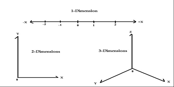
A single dimension can be visualized as a line. Our line has both negative and positive values, which indicate how far we are from the center. Adding a second line, perpendicular to our first, we create a plane. This is the second dimension, typically represented by the x-y plane. If we travel horizontally from our first line, in the direction of our second dimension, our point’s distance from the origin in the first dimension remains unchanged. A point is designated by an ordered pair (typically (x,y)), telling us the point’s position in the first and second dimension, respectively.

If we add a third line, going vertically through the intersection of our first two, we can operate in three dimensions. Our points are now represented by 3-tuples, (x,y,z).

This is all fairly comprehensible. However, linear algebra does not limit itself to 3 dimensions. In fact, it allows us to work with objects in any number of dimensions.

The real space formed by n dimensions is referred to as $ℝ^n$.

Visualizing dimensions greater than three can be difficult. Having four or more perpendicular lines intersect at the same point is impossible within our three-dimensional world. However, even as we venture into higher dimensions, the geometry we know and love still holds. We can still calculate the angle between vectors, find the volume of shapes, and create subspaces.

In higher dimensions, the only difference is that our points contain more information. One helpful way to understand 4+ dimensions is to think of our dimensions as variables in a dataset. For example, in a financial model, you might have nine separate variables for each observation. If we want to measure how these variables relate to one another, we can represent the data in nine-dimensional space and use linear algebra to analyze it.

Throughout the course of this article, I will use examples in $ℝ^2$ and $ℝ^3$, which help with intuition, but are hard to visually extrapolate to higher dimensions.

The following objects are fundamental tools of linear algebra.

A vector is an arrow that encodes a direction and magnitude (length). They are typically represented by a point, where the vector is the arrow from the origin (0,0,…,0) to that point.

A matrix, A, represents a linear transformation, T, an operation we can perform on vectors that preserves vector addition and scaling.

For vectors v and u, and scalars a and b:

I will give a brief explanation of what a matrix is, but for people who want a deeper understanding, watch this incredible video from 3blue1brown. By the way, his video on determinants serves as a nice introduction to what I will talk about, with far better visuals.

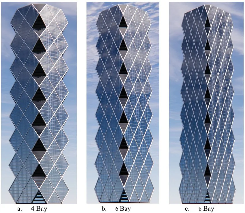
A matrix represents a linear transformation, a function of vectors that outputs exactly one vector for every vector input. They can act between dimensions, corresponding to their length and width (their output and input dimensions, respectively), but in this case, we will focus only on square matrices. A square matrix transforms the coordinate grid into a diagonal grid, preserving lines and linear combinations.

I’m going to assume people understand algebraically how to multiply matrices.

Finally, the dot product (also called the inner product) is an operation we can perform on two vectors within the same dimension. It has two formulas: algebraic and geometric. Typically, we calculate the algebraic formula to derive geometric insight. To calculate the dot product algebraically, we sum the products of the vectors’ terms in each dimension. The geometric way is to multiply the magnitude (length) of the vectors together, and then multiply that by the cosine of the angle between them.

The two most important facts about the dot product are: we can use it to calculate the projections between vectors, and the dot product of perpendicular vectors is zero.

These two facts are related, and if you don’t have intuition for this, take some time to consider how.

Geometric Determinants:

With our mathematical foundation laid, we begin our exploration of determinants with three vectors in 3d space ($ℝ^3$).

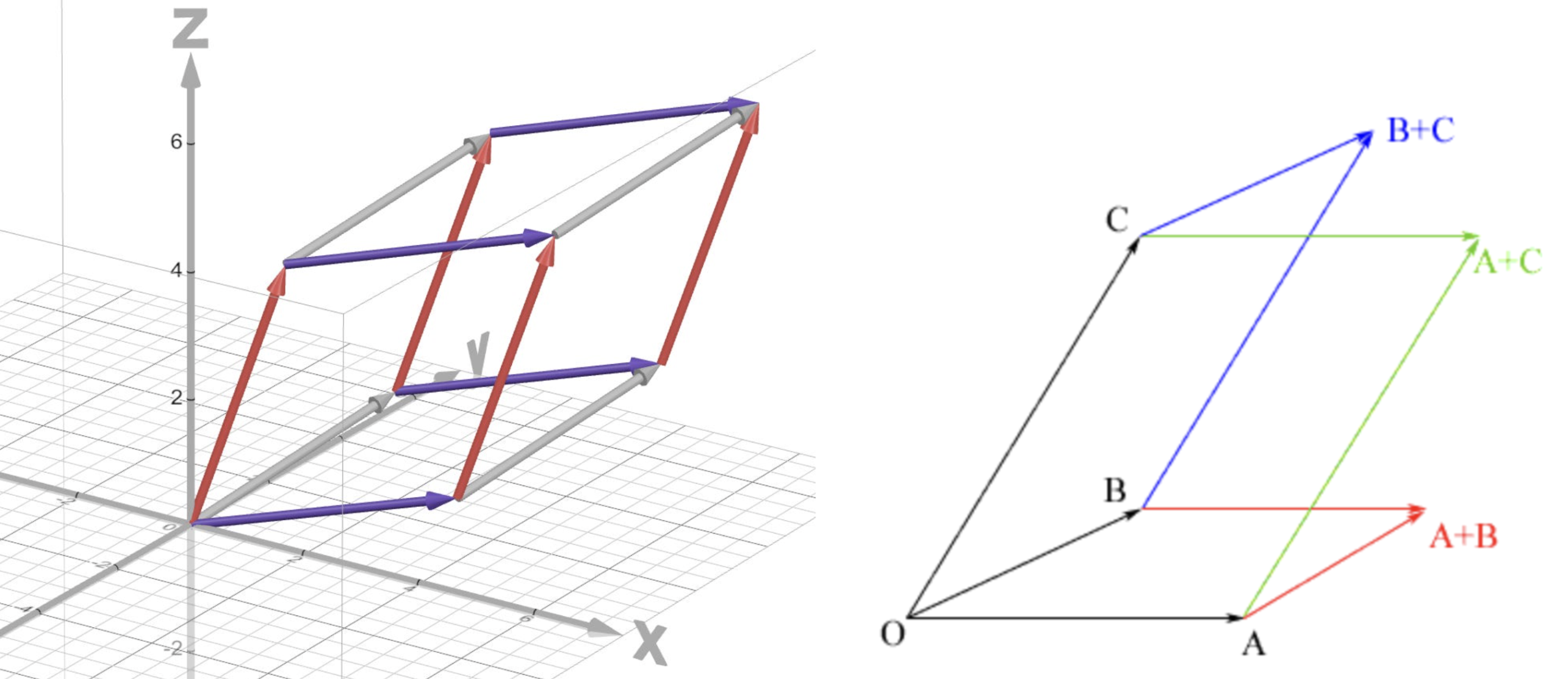
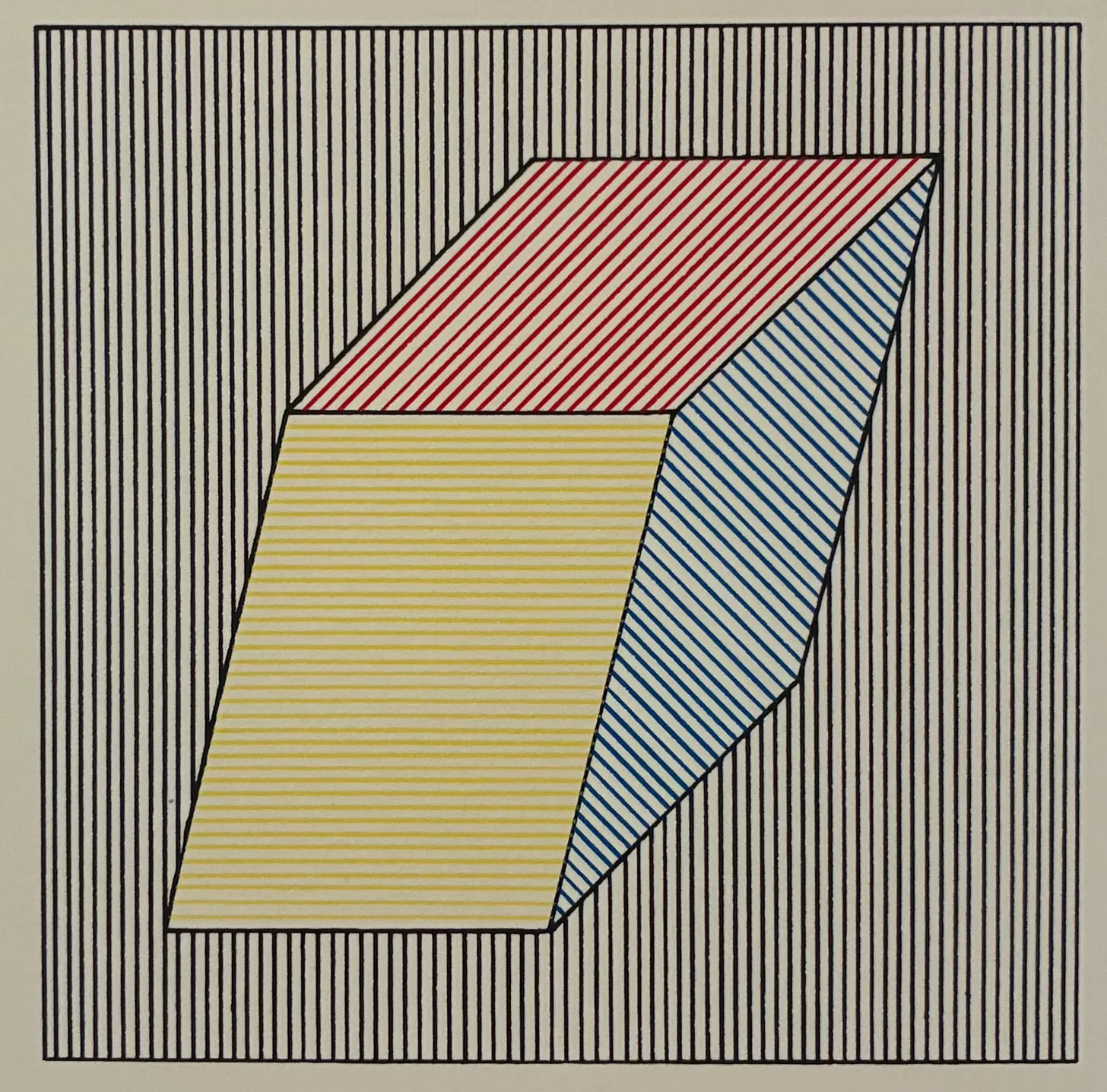
Using these vectors, we form a distorted rectangular prism (a parallelepiped).

If we wish to find the volume of this shape, we could calculate it using geometry. Alternatively, we could use something called a determinant.

The determinant is a number associated with a square matrix. Geometrically, it measures how much the matrix scales volume. We can calculate this number using an algebraic process, which I will explain momentarily, but first, let’s discuss its meaning.

The standard basis is a set of vectors that go one unit in each coordinate direction. In $ℝ^3$, it is ([1,0,0], [0,1,0], [0,0,1]). People refer to these vectors as e1, e2, and e3. For higher dimensions, the standard basis is longer.

In $ℝ^3$, these vectors form a one-by-one-by-one cube, called the unit cube. In $ℝ^2$, they form what is called the unit square, and for higher dimensions, they form what is called the unit hypercube. These objects always have a volume of one. (area/hypervolume in other dimensions)

Consider a 3 by 3 matrix. (Also written as 3 x 3),

If we apply this matrix to the first unit vector, we get the first column:

If we apply it to the second unit vector, we get the second column:

In fact, we can rewrite a matrix based on where it sends our standard basis. (Remember that $e_i$ refers to the ith standard basis vector)

If A is an n x n matrix representing the linear transformation T, then:

We can represent any vector as a linear combination of the standard basis. We can technically do the same with any basis, but the standard basis is simple.

Therefore, if we know how a matrix affects the standard basis, we can determine how it affects any vector.

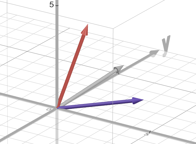
Now, imagine that we want to measure the effect of a matrix on the unit cube itself. To do so, we could form a parallelepiped from the vectors that the elements of our standard basis were mapped to. (ie, our column vectors)

The signed volume of this parallelepiped is the determinant of our matrix.

So how does one calculate a determinant, and why does it give you this fascinating result?

The determinant of a 2x2 matrix A is calculated as follows: (vertical bars on a matrix mean that you are taking the determinant)

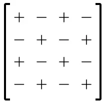
For larger matrices, we start by choosing any row or column. For each value in this set, we multiply it by the determinant of our matrix excluding both the row and column of our value. Finally, we sum these terms together with alternating signs based on the pattern below, which extends correspondingly to larger matrices.

Determinant of a 3x3 matrix row expansion calculation example:

This tells us that the volume of the parallelepiped formed by [1,2,0], [1,1,1], and [0,1,2] is -3. The volume being negative means that at some point, our vectors switched order. This is not insignificant, but for finding the volume, we take the absolute value.

One important aspect of the determinant is that it is multiplicative. That is:

det(AB) = det(A)det(B).

Knowing that the determinant measures scaled volume helps with the intuition here.

Now that we have introduced the determinant, we can move on to the real question. Why does it give you the volume of the transformed unit cube?

For two dimensions, you could verify that the formula matches fairly easily. For three dimensions, you could do this as well, albeit with more calculation. However, doing this for higher dimensions would be tedious and unsatisfying.

For a cleaner proof, we start with the determinant of an n x n matrix.

Let us discuss column addition, which is when you add scaled columns to each other. This action does not change the determinant.

Example:

Here, we subtracted two times our second column from our first column.

To understand why the determinant remains unchanged here, we should think about it in terms of what the determinant is geometrically calculating. That is, the area of the parallelotope formed by our column vectors. As a mathematician, it pains me to use the goal of a proof in the explanation. However, this part is more geometric intuition than a strict proof, and it’s the easiest way to understand it.

(‘Parallelotope’ is the n-dimensional name for the shape of the same family that parallelograms and parallelepipeds belong to.)

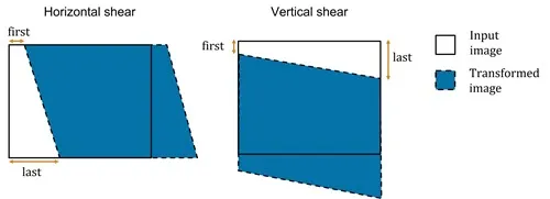
Column addition doesn’t change the volume of our parallelotope because it is a shear.

A shear is an affine transformation that moves all points in a fixed direction based on their distance to a specified line parallel to that direction.

Think of a deck of cards that you nudge at an angle, moving the top ones more than the bottom ones. The important idea: shears do not change volume.

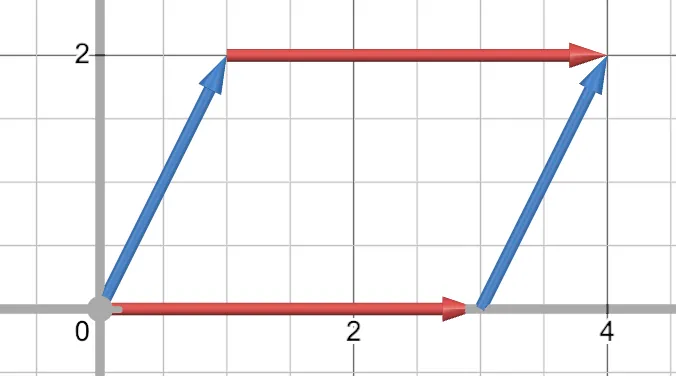
Take vectors [3,0] and [1,2], which form the parallelogram below.

If we subtract from [1,2] a scaled version of [3,0], the top of our parallelogram would remain on the line y = 2. All possible resulting shapes have equal volume.

You could imagine that at some point, our vectors will be perpendicular to each other. At that point, if we want to calculate the area, instead of needing to measure the height of our parallelogram, we can simply multiply the lengths of our vectors together.

With this example, it is easier to adjust [1,2] to be perpendicular to [3,0], as [3,0] lies on an axis. However, we could also go the other way, subtracting scaled versions of [1,2] from [3,0]. With this process, we could also make the vectors perpendicular.

The next step involves generalizing this process to higher dimensions. Thinking about three dimensions, we start with a parallelepiped. As explained, this parallelepiped is formed with three vectors. From these three vectors, we choose any two to act as our base. These two vectors form a parallelogram. Referring to the parallelepiped diagram, you can see that we have three choices for this base.

The goal of this process is to make our vectors perpendicular to each other, without sacrificing volume.

To do so, we start by performing the parallelogram example we just looked at on the two vectors. We make the vectors in the base perpendicular to each other with a shear, subtracting a scaled version of one of them from the other.

Now, we have two perpendicular vectors forming our base, and a final third vector. If we subtract scaled versions of our two base vectors from this third vector, the top moves, while the volume remains constant.

You can imagine that, at some combination of our subtraction, we end up with a third vector perpendicular to both of the vectors that form our base. This set of three perpendicular vectors forms a rectangular prism, with the same volume as our original parallelepiped. This process is visualized below. (Link to Desmos graph)

This process of making our vectors perpendicular can be generalized to n dimensions, and has a name you may have heard before: the Gram-Schmidt process.

Before we generalize this process, it’s important to understand the method of determining how much of each vector to shear when making them perpendicular. We subtract from each vector the amount it travels in the direction of the other vectors. This is a projection, which we can calculate using the dot product. If you want a full breakdown of the Gram-Schmidt process, watch this video from James Hamblin.

For n dimensions, we start by picking a single vector. We then pick a second vector and make it perpendicular to our first. The base at this point is a line, and together the vectors form a rectangle. Next, we pick a third and make it perpendicular to our first two vectors. The base at this point is a rectangle, and together our vectors form a rectangular prism.

For the fourth vector, we do the same thing. We subtract its projection onto our three base vectors, leaving it perpendicular to our base, a parallelepiped. We know this to be true, as if we take the dot product between it and any of our base vectors, we get zero. However, it is essentially impossible to visualize this, as what I’m saying is that we have a vector perpendicular to a three-dimensional object. With that being said, the algebra works; a vector in $ℝ^4$ can be perpendicular to an entire 3-dimensional subspace. One must accept that higher dimensions don’t comply with our understanding of the universe, because we only exist in three.

Moving past that enigmatic fact, we can continue to take new vectors and perpendicularize them until we run out of vectors. This leaves us with an orthogonal set of vectors that form a hyperrectangle with hypervolume equal to our original parallelotope.

Lots of big words. Basically, we make the vectors perpendicular, and now we have a rectangle instead of a parallelogram.

Once we have this new set of vectors, finding the (hyper)volume of our shape is trivial. Because of its rectangular structure, we can determine the volume by multiplying the side lengths of our shape together. In conclusion, we make our vectors perpendicular by subtracting scaled versions of each other, then multiply their magnitudes together to get the volume of our original parallelotope.

Going all the way back to the determinant, we embarked on this whole discussion to prove that we can perform column addition without affecting our determinant’s value. We did so, but also described how we can use column addition to get perpendicular column vectors.

Let’s set up an arbitrary n by n matrix, which we will work with for the remainder of this article. The format below is a way of writing matrices, with $v_1$, $v_2$, etc, as the column vectors.

Perform the Gram-Schmidt process on this matrix’s column vectors, and form another matrix:

As I mentioned, this process uses only column addition, and therefore, the determinants of these two matrices will be the same.

What I will now prove is that the determinant of our matrix U is equal to the magnitudes of its column vectors multiplied together. As we have shown, this product is equal to the volume of the parallelepiped formed by the column vectors of matrix A.

First, we form a new matrix G equal to U transpose times U. The transpose of a matrix is simply the same matrix flipped along its diagonal. This matrix is called a Gram matrix. When we create this matrix, we get the following structure:

If you are confused here, try doing the matrix multiplication yourself.

Because the column vectors of our U matrix are perpendicular to each other, when you take the dot product of two distinct U vectors, you get zero.

The magnitude of a vector is its Euclidean length, calculated using the following formula:

When we take the dot product of a vector with itself, we get its magnitude squared.

We can rewrite our Gram matrix with this in mind.

Keep in mind that the magnitudes of these vectors are the side lengths we use to calculate the volume of our parallelepiped.

Finally, we take the determinant of G. Because it is diagonal, we get the product of its elements.

Now, rewrite the determinant of G in terms of U. This step uses two rules about the determinant: that it is multiplicative, and the determinant of a matrix’s transpose is equal to the determinant of the matrix.

Next, we set our two equations equal to each other.

Take the square root of both sides:

Remember that the determinant of U is equal to the determinant of our original matrix, A.

And with that, we are done! The absolute value of the determinant of a square matrix is equal to the product of the magnitudes of the orthogonal vectors produced by applying Gram-Schmidt to its column vectors.

I hope this made sense. I think it’s very interesting how these ideas, which are taught in linear algebra, are really all connected, but we never learn about them that way. Thank you for reading, and I will catch you in the next edition of this unnamed math blog.

Tay Staviski: We must start by establishing our assumptions. I would formalize our function, as well as the conditions Arrow requires for an ‘optimal’ ranking. Then we can create our optimization algorithm.

Jean Carlé: We won’t be creating the social welfare function, just assuming one exists, though we do need to define its structure. Our inputs are ranked lists of potential outcomes. We take an arbitrary number of outcomes, defined by a group X, and an arbitrary number of voters, defined by a group N. Each member of group N submits an ordinal ranking of all elements in group X. Our social welfare function takes these rankings and outputs an optimal ranking of all outcomes. This ranking most accurately matches the aggregate preferences of group N. Arrow’s Theorem walks through a proof showing that an algorithm of this sort cannot violate the conditions he sets up. To understand how it works properly, we must have a complete understanding of these conditions. May you summarize them for us?

Tay Staviski: The social welfare function must give an output for any set of preferences. Second, this output must reflect all unanimous preferences of our population. Third, the ranking of two variables cannot be influenced by the presence of a third variable. Finally, the decision cannot be determined by the preferences of a single voter.

Jean Carlé: These conditions are respectively called: unrestricted domain, Pareto efficiency, the independence of irrelevant alternatives, and non-dictatorship. Besides these, we assume anonymity, meaning each input is considered equally. Going one by one, I will explain each condition.

Non-dictatorship: This condition states that a sole ‘dictator’ cannot determine the output. A voter acts as a dictator if, for every pair of outcomes, the output reflects the voter’s ranking, no matter what other voters prefer. This condition is assumed with the anonymity of our voters, although Arrow explicitly states non-dictatorship as a factor in his original theorem.

Unrestricted domain: Voters must be able to submit any permutation of outcomes. This ensures our social welfare function actually meets the requirements to be classified as a function. Every possible set of finite voter preferences will be mapped to an output.

Pareto efficiency: Our function’s output must be Pareto efficient. This means that every possible change we could make to our final output will, even if it increases the well-being of one person, decrease the well-being of someone else. In other words, our final output cannot be altered to benefit everyone more. This also means that if our population unanimously prefers an outcome X over Y, that preference must be reflected in our output.

Independence of irrelevant alternatives (IIA): The ranked order between two outcomes in our final output cannot be influenced by the addition or subtraction of another outcome. Theoretically, a third option should not influence a voter’s decision between two outcomes. This condition is necessary for our proof to work.

These conditions are necessary for a fair, rational-choice voting system.

Tay Staviski: If the benefit of some change outweighs the detriment, then should we not still enact the change? Why would we not use a system in which participants assign cardinal variables to each ranking? We could then measure the total well-being for each possible ranking of outcomes, and define an algorithm to determine the exact net effect of changes. The use of ordinal variables significantly reduces our analytical capabilities, as our algorithm cannot account for opinions held by the population, though not unanimously.

Jean Carlé: Pareto efficiency isn’t how we determine our output; it is just a condition that it must fulfill. Our final result does not have to be unanimous, but it must reflect all unanimous preferences our population holds. As to your point of cardinal variables, you are correct that they would allow us to always find the exact result that perfectly optimizes social welfare. However, we run into two key issues. First, cardinal variables aren’t trustworthy for precise measurements of population opinions. If we are using a scale from 1-10, then an outcome that benefits two voters the same amount might be reported as an 8 for one voter and a 10 for another. This discrepancy would happen constantly and would be impossible to account for. Second, take two options: option X being very favorable and option Y being unfavorable. A voter might report 9 for X and 2 for Y, or some other set of similar numbers. Now, imagine a new scenario with the same voter, but options X, Y, and a new, extremely favorable option, Z. The presence of Z does not change the fact that X > Y. This is why IIA holds with ordinal variables. However, if our voter wants to report a 9 for Z, they will most likely lower their number for X. This changes the relative ranking between X and Y. Because cardinal variables mean the introduction of a third outcome might change a voter’s evaluation of two original outcomes, we are forced to use ranked-choice voting. Let us now move on to Arrow’s proof itself.

Arrow’s Impossibility Theorem:

Imagine a scenario with a finite population of size N, and a finite set of outcomes. Among these are two arbitrary and distinct outcomes, X and Y. Assume that we have a unanimous ranking of these two; all participants rank X > Y. We go one by one, and flip each voter’s ranking to Y > X. When all voters rank Y > X, society will as well. Therefore, at some point in this process, we will encounter a pivotal voter, such that flipping their vote will cause society to no longer rank X > Y. We label this voter nxy. When nxy ranks Y > X, we say society ranks Y ≥ X, not the stricter Y > X. This is because it is possible for Y to be equal to X. Similarly, when changing society’s vote from Y > X to X > Y, we can find a voter nyx, who, when ranking X > Y, dictates that society ranks X ≥ Y. With this in mind, we can imagine two possible ways a population N can vote. Label the first S1, and the second S2. We start with a unanimous ranking of X > Y in both, then sequentially flip voters’ opinions to Y > X. In the first group, S1, every voter up until nxy prefers Y > X, while nxy and every subsequent voter prefers X > Y. S2 is the same except for nxy, who prefers Y > X. Therefore, societal ranking is X > Y in S1, and Y ≥ X in S2.

Now we introduce a third outcome, Z, which does not change the relative ranking of X and Y in any way. In S1, all voters place Z directly below Y. By universality, S1 ranks Y > Z. Because X > Y, the societal ranking of S1 is X > Y > Z. Therefore, through transitive property, S1 ranks X > Z even though the vote is not unanimous. In both societies, nxy ranks Z last, below both X and Y. In S2, all voters maintain their relative ranking of X and Z, meaning we keep the societal ranking of X > Z due to IIA. The only change between S1 and S2 among the pairs (X, Y) and (X, Z) is nxy’s pivotal flip. Instead of X > Y > Z (S1), we have Y ≥ X > Z (S2). However, in S2, each voter’s ranking of Y and Z is undefined. This means that each voter could place Z above, equal to, or below Y. This is problematic because, based on our conclusion of Y ≥ X > Z, Y should be above Z. Even though the individual relationship between the outcomes is undefined for each voter, meaning society could rank Z > Y, S2 can never do so. Therefore, with our current setup, Y must be ranked above Z. The only thing that is actually known about the way society ranks the variables is that nxy ranks Y > Z. Next, because IIA says society ranks a pair of outcomes based solely on the way voters rank that pair, we are forced to conclude that when nxy ranks Y > Z, society must rank Y > Z. This is extremely unintuitive, but by the conditions posited, is true.

Let’s imagine all voters in S2 rank Y > Z. We sequentially flip each voter’s ranking to Z > Y in the same way we found nxy. Until we flip nxy, they rank Y > Z, meaning society also ranks Y > Z. Therefore, we must encounter the voter whose ranking of Z > Y invalidates Y > Z after we flip nxy, because while nxy still ranks Y > Z, society can’t change. In other words, nyz ≥ nxy. Next, we repeat this process to find nzy. All voters in S2 rank Z > Y, so society ranks Z > Y. We know that once we flip nxy, society will no longer rank Z > Y. Therefore, nzy must be before or equal to nxy, or nxy ≥ nzy. Putting our two inequalities together, we get: nyz ≥ nxy ≥ nzy. With this, we are almost complete. Remember that our variables are arbitrary and distinct outcomes. Because of this, when we determine a conclusion about them, we would be able to swap their initial positions and therefore know that what we concluded works with a different order of the variables. Think of this not as setting up a new system, but just changing the labels on the same outcomes. Repeating our recent conclusion with Y and Z swapped, we get nzy ≥ nxy ≥ nyz. Using these inequalities together:

nyz ≥ nxy ≥ nzy and nyz ≤ nxy ≤ nzy

We can conclude:

nyz = nxy = nzy

Tay Staviski: Fascinating. At this point, we have proven that a decisive voter for any two outcomes is also a decisive voter for either one of those outcomes and an arbitrary third variable. This clearly extends to a voting pool with any number of outcomes, as repeating this process is trivial. It really is interesting that the whole proof relies on the fact that S2 always conforms to nxy when they rank Y > Z. Especially when that lemma seems to be based on logic, which requires a suspension of belief.

Jean Carlé: This point demonstrates how core Arrow’s axioms are to the proof. They seem so reasonable when introduced that one would assume most voting systems fulfill them. In reality, they are seldom realized entirely. Because this proof’s logic stretches its conditions to their absolute limit, any margin for error on a factor such as IIA would invalidate the proof entirely. In modern politics, people use this proof as an argument against ranked-choice voting systems, when there is little to no chance that even small elections could be done while ensuring IIA completely. Arrow’s theory reminds us to heavily prepare before attempting to prove something. It is a foundational piece of math, and its limited real-world application should not diminish its respect. It is a proof which has been re-written, taken out of context, and misused possibly more than any other in history, and will continue to be used in this way. Understanding its true mechanisms gives a slight shock, and at the very least, allows one to skepticize people quoting it in ways you now know to be invalid. Thank you for listening.

How could we define this library from a mathematical standpoint? The simlplest case, though we would lose information, is that of a standard alphabet and size. Let’s say we have 32 characters, each letter in the English alphabet, along with some basic punctuation symbols: (, . : ? ; space). We’re skipping quite a lot here, such as all of mathematics. However, with this set, it’s not unreasonable to claim that most information is conveyable.

In the original story, each book has a standard template: 410 pages, 40 lines on each page, and 80 characters in each line. We can imagine a library that contains all possible combinations of characters needed to fill this book. This library would be unimaginably massive, with the number of possible books having over 2 million digits, assuming there are no repetitions. Given, most of these would consist of nothing but random letters. However, it would also contain exact copies of all books written with less than 1.6 million characters, and variations of each with one-character differences. It contains all possible iterations of ASCII art, and therefore copies of every painting made with symbols.

Let’s abstract this a bit, stepping away from the story itself. It would be better not to have a limit on the number of characters we can put, so let’s do just that. We still have constraints, namely the fact that while the books themselves can be any size, they still must be finite. This new library would be truly infinite, but would still be countable, due to our defined number of characters. To create a correspondence between this library and the natural numbers, we could assign an order to our characters, then order our books as such:

1,1,1,1… 1

1,1,1,1… 2

…

1,1,1,1… 32

1,1,1,1… 2, 1

1,1,1,1… 2, 2

…

1,1,1,1… 2, 32

1,1,1,1… 3, 1

…

1,1,1,1… 32, 32

1,1,1,1… 2, 1, 1

…

32, 32, 32… 32

This is similar to counting in base 32. With this, we can establish a correspondence with the natural numbers, meaning the number of books is countably infinite.

So how would we organize the library when accepting books of any alphabet? We could use Paul Dancstep’s presentation of the library. For each combination of a number of characters and a number of spaces we can put them in, we create a collection of possible books.

We can organize these collections in a grid pattern, with the block closest to the origin using an alphabet with 1 character and having 1 space for it to go. One axis is the number of characters, and the other is the number of spaces. This grid is filled with blocks, which are collections of the possible books that can be in them. We can create a clear mapping between the structure of these categories and the x-y plane, and therefore, the number of categories is countable. Additionally, each collection will contain a finite number of books, so we can conclude that this new library is still countable.

One thing which we have overlooked is the order of characters, which is necessary for us to order the books within these categories. We can order each collection with the same process we used to count the books earlier, allowing us to call books directly. We could imagine a distinct vector that allows us to find the exact book we want with three distinct variables: alphabet length, book length, and the index within each collection. This is a useful way to index our library, though it is limited. To perform any analysis of a book, we would have to return to our model and find the structure of the book we are referencing. Also, we would be unable to perform operations between the vectors themselves, as they only act as an index. For the purpose of this essay, we want to try and find something generalizable to linear algebra, in which we have a very established framework for the interaction between vectors. While our current model does index books as vectors, we can’t perform actions such as matrix multiplication or addition. Let’s try another approach which uses linear algebra.

Before we do so, we have to slightly shift our focus. Exploring our infinite library has led us to a deeper task: quantifying langauge. We must break down the books into paragraphs, sentences, words, and even morphemes (pre, anti, etc.). Therefore, when moving forward, we will keep the same structure of the library in mind, but instead of thinking of books in their entirety, we will think of short words with much smaller amounts of characters. Another point: while we wish we could use every language format, there are different meanings for the same symbols across languages. Therefore, it will be extremely difficult to derive meaning unless we decide on a specific language. We can even generalize our format so it works with any language, but once we choose one, we can’t switch interchangeably. For now we may stick to english.

Instead of trying to fit an index of the books into a vector, we can build the system from the basis. We will avoid the generalization of languages for now and focus on defining a vector space for each possible alphabet. This way, we can represent words as vectors, and in this vector space perform interactions between them, allowing us to interpret them mathematically. For example, say we have a collection of books with 5 possible characters. We can establish a basis from these characters as such:

[1, 0, 0, 0, 0] for A

[0, 1, 0, 0 ,0] for B

[0, 0, 1, 0, 0] for C

[0, 0, 0, 1, 0] for D

[0, 0, 0, 0 ,1] for L

We can generalize this format to languages with any number of characters, simply adding more bases. Now, when making a book, sentence, or word, we can put together these rows in a matrix. For example, CABAL would look like such:

[0, 0, 1, 0, 0]

[1, 0, 0, 0, 0]

[0, 1, 0, 0, 0]

[1, 0, 0, 0, 0]

[0, 0, 0, 0, 1]

This is interesting, and now we have strings represented in a matrix, though when putting them together we might need to add a space into our set of characters. However, this is not that practical, especially if we want to represent something as long as a full book. As of now, we have little more than a simple cipher. But this structure is the building block of more complicated mathematical representations of language. Let’s discuss embedding.

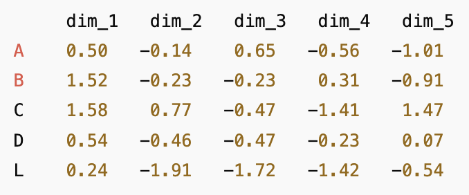
One of the most prevalent cases of language-to-math conversion is AI and the study of natural language processing. However, they don’t observe texts using this one-hot vector form. This form allows us to represent each character as a vector, but it is rigid and mostly uninformative, not telling us anything about how one character relates to another. Therefore, an AI encodes words using an embedding matrix. An embedding matrix defines, for each of our characters, a specific number that determines the placement of that character. It might be easier to work with an example:

General form:

[a1, a2, a3, a4, a5]

[b1, b2, b3, b4, b5]

[c1, c2, c3, c4, c5]

[d1, d2, d3, d4, d5]

[l1, l2, l3, l4, l5]

Our word cabal might look like:

Each row is a 5-dimensional embedding for the corresponding character. We can use this to express a word as a matrix of embedded vectors. One important caveat here is that while this form is usually discussed as a matrix, it is more akin to a list of vectors for each letter, which when combined act as a matrix. When referencing a word, AI needs not only the letters comprising it, but also the context surrounding their usage. In this form, the rows determine the letter order, and we still have the other information about weights.

These weights are not random, they are chosen by AI systems to represent the use of those characters in the position which each weight refers to. The weights are generally not readable by humans, or at least we have little to no intuition surrounding them. AI models are trained to create these weights. To understand this further, we need to break down the way AI models work, and how they are trained.

AI is trained by human input in the form of pre-labeled sentences which contain meaning. Sometimes, this meaning is made explicit, as would be the case with early stage development, using small sets of sorted data. However, it could also assume this implicitly, such as when training on huge sets of data such as the internet. Without this training, an AI has no way to distinguish real words from random combinations of letters.

This system is different from the way humans learn, but there are many parallels to be drawn, and without training of our own, humans are similarly incapable of deciphering meaning. If a human were to walk around the Library of Babel, and pick books to read at random, almost every time they would encounter nothing but random strings of letters. However, If a book you pick up happens to be a real story written in English, I, or someone similar, would recognize it as containing meaning. This decision would be based on prior knowledge and understanding of the English language. If there was a book written in a language you had no knowledge of, you would have a very difficult time differentiating it from something meaningless, or random letters. In the same way, a human who somehow had no knowledge of written language in any form would have no idea what anything in the library means, including books written in English.

Before training, AI acts similarly to someone like this, with no knowledge of how sentences are put together. When it is trained with human labeled data, it recalibrates its weights to fit the real examples of meaning. For example, an AI might receive a sentence such as

“The cat slept on the ___.”

It would then attempt to guess what the last word might be. To do this, it would use the weights and determine what it believes is most likely to conclude the sentence, based on past data it has seen. Let’s say the AI decided on “roof”, though the actual answer was “mat”. It would then compare the response it gave, calculating the dot product between its proposed answer and the correct answer. Then, it changes its weights, altering its prediction matrices to incorporate the error. Through this process, an AI develops its embedding matrix, which is used to discern the probabilities of words being used in the context of their surroundings. Advanced models are trained on unimaginable amounts of data, which is what allows it to be so accurate to human speech. Additionally, they can determine when specific kinds of responses are appropriate, for example when prompted to respond casually versus academically, they have different probability matrices for the way they decide their words.

Before we link AI back to our infinite library, let’s finish our explanation of how it works. When an AI is reading a sentence, as much as we would like it to be the case, it doesn’t just generate an embedded sequence of matrices for each word. First, it breaks down the sentence into tokens, which are normally words, but can be meaningful subsections of words as well. It then assigns positional matrices, which tell the AI the order in which the tokens are organized. Then, it sends the tokens through its constructed embedding matrix, and outputs them as embedded vectors. So the example I gave earlier is not entirely representative, most of the time a sentence will be represented as a list of embedded vectors corresponding to each word. The length of an embedded vector is dependent on the sophistication of the language model being used, as it is what the AI uses to encode meaning. This length can range from dozens to thousands. So the full process is as such: tokenization → embedding matrix → positional matrix.

Let’s explore how an AI might be able to help us organize our library of babel. If we are starting with a completely untrained AI, it would be even more lost than us, as even if it encountered sensible text it would not know what it meant. However, let’s say in addition to the AI we had a human interpreter. The AI could bring to this person books it believes to be containing real text, and have them assess its classification. Over time, by recognizing patterns in the books it brings which contain real information, the AI would gradually train itself. After enough time has passed, it will be able to correctly distinguish between sense and nonsense with some level of acceptable accuracy. We could then have this AI read as much of the library as possible, and return with the collection of books it deems to be sensible. This is a possible method of sorting the library, and probably one of the more efficient ones.

When Borges originally wrote his short story pertaining to this library, it was laced with futility, as he believed that the library was unexplorable to a meaningful extent. He begins the story with hope for the utility of the library, but as the characters explore the library, the amount of useless data becomes insurmountable. The number of books is truly infinite, and therefore, the number of illogical books is infinite as well, along with the number of logical ones. However, with the method described using AI, we can observe a very large number of books, arguably any finite number given enough time. Therefore, depending on how the library is organized, we could imagine sorting all books under a certain specific length. This throws the pessimistic view of the library from borges into question, as even if we can’t truly look through each and every book, we can find some extremely interesting things. There’s so many more questions to ask, and we haven’t even begun to delve into many of the interesting philosophical ramifications of having such a library, which was the main focus of the original story. However we have used it as an excuse to mathematically interpret language and explain an interesting technology, which I think is pretty cool. Thanks for reading!