Geometric Determinants

What is a determinant? You may have used the operation before, but do you know what it means? If you do know what it means, do you know the explanation behind it? This article will discuss the true meaning behind determinants, framed around finding the volume of a parallelepiped constructed by three vectors. This article will assume a baseline level of linear algebra knowledge. However, the following preface will explain the key ideas used, so hopefully those interested will be able to follow.

Preface:

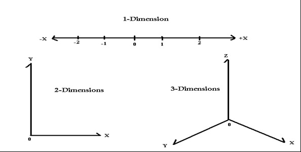
A single dimension can be visualized as a line. Our line has both negative and positive values, which indicate how far we are from the center. Adding a second line, perpendicular to our first, we create a plane. This is the second dimension, typically represented by the x-y plane. If we travel horizontally from our first line, in the direction of our second dimension, our point’s distance from the origin in the first dimension remains unchanged. A point is designated by an ordered pair (typically (x,y)), telling us the point’s position in the first and second dimension, respectively.

If we add a third line, going vertically through the intersection of our first two, we can operate in three dimensions. Our points are now represented by 3-tuples, (x,y,z).

This is all fairly comprehensible. However, linear algebra does not limit itself to 3 dimensions. In fact, it allows us to work with objects in any number of dimensions.

The real space formed by n dimensions is referred to as $ℝ^n$.

Visualizing dimensions greater than three can be difficult. Having four or more perpendicular lines intersect at the same point is impossible within our three-dimensional world. However, even as we venture into higher dimensions, the geometry we know and love still holds. We can still calculate the angle between vectors, find the volume of shapes, and create subspaces.

In higher dimensions, the only difference is that our points contain more information. One helpful way to understand 4+ dimensions is to think of our dimensions as variables in a dataset. For example, in a financial model, you might have nine separate variables for each observation. If we want to measure how these variables relate to one another, we can represent the data in nine-dimensional space and use linear algebra to analyze it.

Throughout the course of this article, I will use examples in $ℝ^2$ and $ℝ^3$, which help with intuition, but are hard to visually extrapolate to higher dimensions.

The following objects are fundamental tools of linear algebra.

A vector is an arrow that encodes a direction and magnitude (length). They are typically represented by a point, where the vector is the arrow from the origin (0,0,…,0) to that point.

A matrix, A, represents a linear transformation, T, an operation we can perform on vectors that preserves vector addition and scaling.

For vectors v and u, and scalars a and b:

\[T(a \mathbf v + b \mathbf u) = aT( \mathbf v) + bT(\mathbf u)\]

I will give a brief explanation of what a matrix is, but for people who want a deeper understanding, watch this incredible video from 3blue1brown. By the way, his video on determinants serves as a nice introduction to what I will talk about, with far better visuals.

A matrix represents a linear transformation, a function of vectors that outputs exactly one vector for every vector input. They can act between dimensions, corresponding to their length and width (their output and input dimensions, respectively), but in this case, we will focus only on square matrices. A square matrix transforms the coordinate grid into a diagonal grid, preserving lines and linear combinations.

I’m going to assume people understand algebraically how to multiply matrices.

Finally, the dot product (also called the inner product) is an operation we can perform on two vectors within the same dimension. It has two formulas: algebraic and geometric. Typically, we calculate the algebraic formula to derive geometric insight. To calculate the dot product algebraically, we sum the products of the vectors’ terms in each dimension. The geometric way is to multiply the magnitude (length) of the vectors together, and then multiply that by the cosine of the angle between them.

\[\mathbf u \cdot \mathbf v = u_1 v_1 + u_2 v_2 + ... + u_1 v_1 = ||\mathbf u || || \mathbf v || \cos (\theta)\]

The two most important facts about the dot product are: we can use it to calculate the projections between vectors, and the dot product of perpendicular vectors is zero.

These two facts are related, and if you don’t have intuition for this, take some time to consider how.

Geometric Determinants:

With our mathematical foundation laid, we begin our exploration of determinants with three vectors in 3d space ($ℝ^3$).

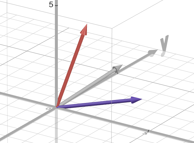
Using these vectors, we form a distorted rectangular prism (a parallelepiped).

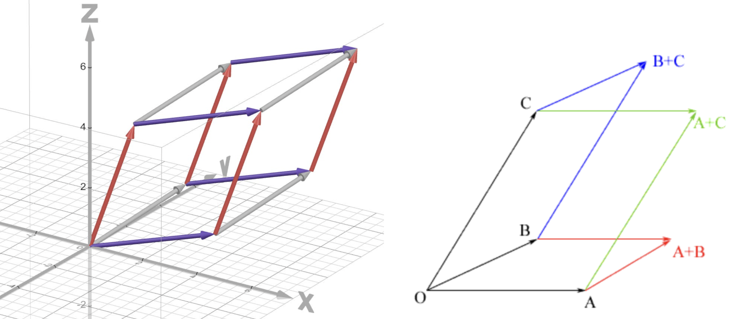
If we wish to find the volume of this shape, we could calculate it using geometry. Alternatively, we could use something called a determinant.

The determinant is a number associated with a square matrix. Geometrically, it measures how much the matrix scales volume. We can calculate this number using an algebraic process, which I will explain momentarily, but first, let’s discuss its meaning.

The standard basis is a set of vectors that go one unit in each coordinate direction. In $ℝ^3$, it is ([1,0,0], [0,1,0], [0,0,1]). People refer to these vectors as e1, e2, and e3. For higher dimensions, the standard basis is longer.

In $ℝ^3$, these vectors form a one-by-one-by-one cube, called the unit cube. In $ℝ^2$, they form what is called the unit square, and for higher dimensions, they form what is called the unit hypercube. These objects always have a volume of one. (area/hypervolume in other dimensions)

Consider a 3 by 3 matrix. (Also written as 3 x 3),

\[\begin{bmatrix} a & b & c \\ d & e & f \\ g & h & i \end{bmatrix}\]

If we apply this matrix to the first unit vector, we get the first column:

\[\begin{bmatrix} a & b & c \\ d & e & f \\ g & h & i \end{bmatrix} \begin{bmatrix} 1 \\ 0 \\ 0 \end{bmatrix} = \begin{bmatrix} a \\ d \\ g \end{bmatrix}\]

If we apply it to the second unit vector, we get the second column:

\[\begin{bmatrix} a & b & c \\ d & e & f \\ g & h & i \end{bmatrix} \begin{bmatrix} 0 \\ 1 \\ 0 \end{bmatrix} = \begin{bmatrix} b \\ e \\ h \end{bmatrix}\]

In fact, we can rewrite a matrix based on where it sends our standard basis. (Remember that $e_i$ refers to the ith standard basis vector)

If A is an n x n matrix representing the linear transformation T, then:

\[A = \begin{bmatrix} \vert & \vert & & \vert \\ T(e_1) & T(e_2) & ... & T(e_n) \\ \vert & \vert & & \vert \end{bmatrix}\]

We can represent any vector as a linear combination of the standard basis. We can technically do the same with any basis, but the standard basis is simple.

\[\begin{bmatrix} 3 \\ 4 \end{bmatrix} = 3 \begin{bmatrix} 1 \\ 0 \end{bmatrix} + 4\begin{bmatrix} 0\\ 1 \end{bmatrix} = 3 e_1 + 4 e_2\]

Therefore, if we know how a matrix affects the standard basis, we can determine how it affects any vector.

\[T(\begin{bmatrix} 3 \\ 4 \end{bmatrix}) = 3 T(e_1) + 4T(e_2)\]

Now, imagine that we want to measure the effect of a matrix on the unit cube itself. To do so, we could form a parallelepiped from the vectors that the elements of our standard basis were mapped to. (ie, our column vectors)

The signed volume of this parallelepiped is the determinant of our matrix.

So how does one calculate a determinant, and why does it give you this fascinating result?

The determinant of a 2x2 matrix A is calculated as follows: (vertical bars on a matrix mean that you are taking the determinant)

\[A = \begin{bmatrix} a & b \\ c & d \end{bmatrix} \hspace{1cm} det(A) = \begin{vmatrix} a & b \\ c & d \end{vmatrix} = (ad - bc)\]

For larger matrices, we start by choosing any row or column. For each value in this set, we multiply it by the determinant of our matrix excluding both the row and column of our value. Finally, we sum these terms together with alternating signs based on the pattern below, which extends correspondingly to larger matrices.

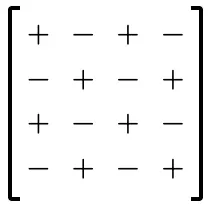
Determinant of a 3x3 matrix row expansion calculation example:

\[\{\mathbf v_1, \mathbf v_2, \mathbf v_3\} = \{\begin{bmatrix} 1\\ 2\\ 0 \end{bmatrix}, \begin{bmatrix} 1\\ 1\\ 1 \end{bmatrix}, \begin{bmatrix} 0 \\ 1 \\ 2 \end{bmatrix} \} \hspace{1cm} A = \begin{bmatrix} 1 & 1 & 0 \\ 2 & 1 & 1 \\ 0 & 1 & 2 \end{bmatrix}\] \[\det(A) = \begin{vmatrix} 1 & 1 & 0 \\ 2 & 1 & 1 \\ 0 & 1 & 2 \end{vmatrix} = 1 \begin{vmatrix} 1 & 1 \\ 1 & 2 \end{vmatrix} - 1 \begin{vmatrix} 2 & 1 \\ 0 & 2 \end{vmatrix} + 0 \begin{vmatrix} 2 & 1 \\ 0 & 1 \end{vmatrix}\] \[=1(1*2 - 1*1) - 1(2*2 - 1*0) + 0= (2-1) - (4) = -3\]

This tells us that the volume of the parallelepiped formed by [1,2,0], [1,1,1], and [0,1,2] is -3. The volume being negative means that at some point, our vectors switched order. This is not insignificant, but for finding the volume, we take the absolute value.

One important aspect of the determinant is that it is multiplicative. That is:

det(AB) = det(A)det(B).

Knowing that the determinant measures scaled volume helps with the intuition here.

Now that we have introduced the determinant, we can move on to the real question. Why does it give you the volume of the transformed unit cube?

For two dimensions, you could verify that the formula matches fairly easily. For three dimensions, you could do this as well, albeit with more calculation. However, doing this for higher dimensions would be tedious and unsatisfying.

For a cleaner proof, we start with the determinant of an n x n matrix.

Let us discuss column addition, which is when you add scaled columns to each other. This action does not change the determinant.

Example:

\[\begin{vmatrix} 3 & 1 & 0 \\ 4 & 2 & 0 \\ 2 & 0 & 1 \end{vmatrix} = \begin{vmatrix} (3 - 2)& 1 & 0 \\ (4-4) & 2 & 0 \\ (2-0) & 0 & 1 \end{vmatrix} = \begin{vmatrix} 1 & 1 & 0 \\ 0 & 2 & 0 \\ 2 & 0 & 1 \end{vmatrix}\]

Here, we subtracted two times our second column from our first column.

To understand why the determinant remains unchanged here, we should think about it in terms of what the determinant is geometrically calculating. That is, the area of the parallelotope formed by our column vectors. As a mathematician, it pains me to use the goal of a proof in the explanation. However, this part is more geometric intuition than a strict proof, and it’s the easiest way to understand it.

(‘Parallelotope’ is the n-dimensional name for the shape of the same family that parallelograms and parallelepipeds belong to.)

Column addition doesn’t change the volume of our parallelotope because it is a shear.

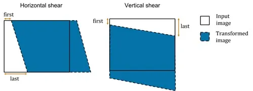
A shear is an affine transformation that moves all points in a fixed direction based on their distance to a specified line parallel to that direction.

Think of a deck of cards that you nudge at an angle, moving the top ones more than the bottom ones. The important idea: shears do not change volume.

Take vectors [3,0] and [1,2], which form the parallelogram below.

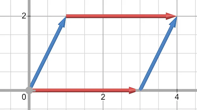
If we subtract from [1,2] a scaled version of [3,0], the top of our parallelogram would remain on the line y = 2. All possible resulting shapes have equal volume.

You could imagine that at some point, our vectors will be perpendicular to each other. At that point, if we want to calculate the area, instead of needing to measure the height of our parallelogram, we can simply multiply the lengths of our vectors together.

With this example, it is easier to adjust [1,2] to be perpendicular to [3,0], as [3,0] lies on an axis. However, we could also go the other way, subtracting scaled versions of [1,2] from [3,0]. With this process, we could also make the vectors perpendicular.

The next step involves generalizing this process to higher dimensions. Thinking about three dimensions, we start with a parallelepiped. As explained, this parallelepiped is formed with three vectors. From these three vectors, we choose any two to act as our base. These two vectors form a parallelogram. Referring to the parallelepiped diagram, you can see that we have three choices for this base.

The goal of this process is to make our vectors perpendicular to each other, without sacrificing volume.

To do so, we start by performing the parallelogram example we just looked at on the two vectors. We make the vectors in the base perpendicular to each other with a shear, subtracting a scaled version of one of them from the other.

Now, we have two perpendicular vectors forming our base, and a final third vector. If we subtract scaled versions of our two base vectors from this third vector, the top moves, while the volume remains constant.

You can imagine that, at some combination of our subtraction, we end up with a third vector perpendicular to both of the vectors that form our base. This set of three perpendicular vectors forms a rectangular prism, with the same volume as our original parallelepiped. This process is visualized below. (Link to Desmos graph)

This process of making our vectors perpendicular can be generalized to n dimensions, and has a name you may have heard before: the Gram-Schmidt process.

Before we generalize this process, it’s important to understand the method of determining how much of each vector to shear when making them perpendicular. We subtract from each vector the amount it travels in the direction of the other vectors. This is a projection, which we can calculate using the dot product. If you want a full breakdown of the Gram-Schmidt process, watch this video from James Hamblin.

For n dimensions, we start by picking a single vector. We then pick a second vector and make it perpendicular to our first. The base at this point is a line, and together the vectors form a rectangle. Next, we pick a third and make it perpendicular to our first two vectors. The base at this point is a rectangle, and together our vectors form a rectangular prism.

For the fourth vector, we do the same thing. We subtract its projection onto our three base vectors, leaving it perpendicular to our base, a parallelepiped. We know this to be true, as if we take the dot product between it and any of our base vectors, we get zero. However, it is essentially impossible to visualize this, as what I’m saying is that we have a vector perpendicular to a three-dimensional object. With that being said, the algebra works; a vector in $ℝ^4$ can be perpendicular to an entire 3-dimensional subspace. One must accept that higher dimensions don’t comply with our understanding of the universe, because we only exist in three.

Moving past that enigmatic fact, we can continue to take new vectors and perpendicularize them until we run out of vectors. This leaves us with an orthogonal set of vectors that form a hyperrectangle with hypervolume equal to our original parallelotope.

Lots of big words. Basically, we make the vectors perpendicular, and now we have a rectangle instead of a parallelogram.

Once we have this new set of vectors, finding the (hyper)volume of our shape is trivial. Because of its rectangular structure, we can determine the volume by multiplying the side lengths of our shape together. In conclusion, we make our vectors perpendicular by subtracting scaled versions of each other, then multiply their magnitudes together to get the volume of our original parallelotope.

Going all the way back to the determinant, we embarked on this whole discussion to prove that we can perform column addition without affecting our determinant’s value. We did so, but also described how we can use column addition to get perpendicular column vectors.

Let’s set up an arbitrary n by n matrix, which we will work with for the remainder of this article. The format below is a way of writing matrices, with $v_1$, $v_2$, etc, as the column vectors.

\[A = \begin{bmatrix} \vert & \vert & & \vert \\ \mathbf v_1 & \mathbf v_2 & ... & \mathbf v_n\\ \vert & \vert & & \vert \end{bmatrix}\]

Perform the Gram-Schmidt process on this matrix’s column vectors, and form another matrix:

\[U = \begin{bmatrix} \vert & \vert & & \vert \\ \mathbf u_1 & \mathbf u_2 & ... & \mathbf u_n\\ \vert & \vert & & \vert \end{bmatrix}\]

As I mentioned, this process uses only column addition, and therefore, the determinants of these two matrices will be the same.

What I will now prove is that the determinant of our matrix U is equal to the magnitudes of its column vectors multiplied together. As we have shown, this product is equal to the volume of the parallelepiped formed by the column vectors of matrix A.

First, we form a new matrix G equal to U transpose times U. The transpose of a matrix is simply the same matrix flipped along its diagonal. This matrix is called a Gram matrix. When we create this matrix, we get the following structure:

\[G = \begin{bmatrix} \text{---} & \mathbf u_1 & \text{---} \\ \text{---} & \mathbf u_2 & \text{---} \\ & ... & \\ \text{---} & \mathbf u_n & \text{---} \end{bmatrix} \begin{bmatrix} \vert & \vert & & \vert \\ \mathbf u_1 & \mathbf u_2 & ... & \mathbf u_n\\ \vert & \vert & & \vert \end{bmatrix}\] \[G = \begin{bmatrix} \mathbf u_1\cdot \mathbf u_1 & \mathbf u_1 \cdot \mathbf u_2 & ... & \mathbf u_1 \cdot \mathbf u_n \\ \mathbf u_2 \cdot \mathbf u_1 & \mathbf u_2 \cdot \mathbf u_2 & ... & \mathbf u_2 \cdot \mathbf u_n \\ ... & ... & ... & ... \\ \mathbf u_n \cdot \mathbf u_1 & \mathbf u_n \cdot \mathbf u_2 & ... & \mathbf u_n \cdot \mathbf u_n \end{bmatrix}\]

If you are confused here, try doing the matrix multiplication yourself.

Because the column vectors of our U matrix are perpendicular to each other, when you take the dot product of two distinct U vectors, you get zero.

\[G = \begin{bmatrix} \mathbf u_1 \cdot \mathbf u_1 & 0 & ... & 0 \\ 0 & \mathbf u_2 \cdot \mathbf u_2 & ... & 0 \\ ... & ... & ... & ... \\ 0 & 0 & ... & \mathbf u_n \cdot \mathbf u_n \end{bmatrix}\]

The magnitude of a vector is its Euclidean length, calculated using the following formula:

\[\mathbf u = \begin{bmatrix} u_1 \\ u_2 \\ ... \\ u_n \end{bmatrix} \hspace{1cm} || \mathbf u || = \sqrt{u_1 ^ 2 + u_2 ^ 2 + ... + u_n^2}\]

When we take the dot product of a vector with itself, we get its magnitude squared.

\[\mathbf u \cdot \mathbf u = u_1^2 + u_2^2 + ... + u_n^2 = ||\mathbf u || ^2\]

We can rewrite our Gram matrix with this in mind.

\[G = \begin{bmatrix} ||\mathbf u_1||^2 & 0 & ... & 0 \\ 0 & ||\mathbf u_2||^2 & ... & 0 \\ ... & ... & ... & ... \\ 0 & 0 & ... & ||\mathbf u_n||^2 \end{bmatrix}\]

Keep in mind that the magnitudes of these vectors are the side lengths we use to calculate the volume of our parallelepiped.

Finally, we take the determinant of G. Because it is diagonal, we get the product of its elements.

\[\det(G) = ||\mathbf u_1 || ^2 ||\mathbf u_2||^2 ... ||\mathbf u_n||^2 = (||\mathbf u_1 || ||\mathbf u_2|| ... ||\mathbf u_n||)(||\mathbf u_1 || ||\mathbf u_2||... ||\mathbf u_n||)\]

Now, rewrite the determinant of G in terms of U. This step uses two rules about the determinant: that it is multiplicative, and the determinant of a matrix’s transpose is equal to the determinant of the matrix.

\[\det(G) = \det(U^T U) = \det(U^T)\det(U) = \det(U)^2\]

Next, we set our two equations equal to each other.

\[\det(U)^2 = (||\mathbf u_1 || ||\mathbf u_2|| ... ||\mathbf u_n||)(||\mathbf u_1 || ||\mathbf u_2|| ... ||\mathbf u_n||)\]

Take the square root of both sides:

\[\lvert \det(U) \rvert = ||\mathbf u_1 || ||\mathbf u_2|| ... ||\mathbf u_n||\]

Remember that the determinant of U is equal to the determinant of our original matrix, A.

And with that, we are done! The absolute value of the determinant of a square matrix is equal to the product of the magnitudes of the orthogonal vectors produced by applying Gram-Schmidt to its column vectors.

I hope this made sense. I think it’s very interesting how these ideas, which are taught in linear algebra, are really all connected, but we never learn about them that way. Thank you for reading, and I will catch you in the next edition of this unnamed math blog.